Robust Statistical Comparison of Classifiers Using the Friedman Test
Introduction
The objective of this assignment is to perform a robust statistical comparison of multiple machine learning classifiers across several independent datasets. When evaluating more than two models over multiple datasets, traditional parametric tests such as the Analysis of Variance (ANOVA) are often unsuitable. This is because the assumptions of a normal distribution and homogeneity of variance are frequently violated by classification accuracy scores. To address this, we employ the Friedman test, a non-parametric (distribution-free) alternative, which rather than analyzing raw performance scores, operates on the relative ranks of the algorithms.
The Friedman Test Statistic
Let $N$ denote the total number of datasets and $k$ the number of classifiers being compared. The procedure begins by ranking the $k$ classifiers on each individual dataset based on their performance metric (assigning average ranks in the case of ties).
Under the null hypothesis, which assumes that all algorithms are equivalent and their performance differences are merely due to random chance, the expected average rank for each classifier is $(k+1)/2$. The test determines whether the observed average ranks diverge significantly from this expected value.
Let $R_j$ represent the average rank of the $j$-th algorithm across all $N$ datasets. The original Friedman test statistic assesses the variance of the average ranks from this expected value and is defined as: $$ \chi_{F}^{2} = \frac{12 N}{k(k+1)} \left[ \sum_{j=1}^{k} R_j^2 - \frac{k(k+1)^2}{4} \right] $$
This statistic is distributed according to the Chi-square distribution with $k-1$ degrees of freedom.
If the p-value associated with the test statistic falls below the chosen significance level (typically $\alpha = 0.05$), we reject the null hypothesis, concluding that at least one classifier’s performance differs significantly from the rest. However, the Friedman test only indicates the presence of a significant difference globally; it does not identify which specific algorithms differ. To pinpoint these exact pairwise differences, we must proceed with a post-hoc procedure.
Nemenyi Post-Hoc Test
Once the Friedman test has rejected the null hypothesis, the Nemenyi test is widely used to compare all classifiers against each other. The Nemenyi test states that the performance of two classifiers $i$ and $j$ is significantly different if the absolute difference $|R_i - R_j|$ between their average ranks is equal to or strictly greater than a threshold known as the Critical Difference:
$$ C D = q_{\alpha} \sqrt{\frac{k(k+1)}{6N}} $$
Here, $q_{\alpha}$ represents the critical value based on the Studentized range statistic divided by $\sqrt{2}$, which depends on the significance level $\alpha$ and the number of classifiers $k$.
Motivation for the Resampling Strategy
Before we can calculate the aforementioned ranks and apply the Friedman and Nemenyi tests, we must first obtain accurate and unbiased performance estimates for each classifier on every dataset. While the non-parametric tests dictate how we compare scores across datasets, we also need a reliable evaluation protocol to measure the models’ performance within each dataset. A standard 10-fold cross-validation often suffers from overlapping training sets, which violates the assumption of independence required for rigorous statistical testing and inflates the probability of false positives. Therefore, we perform a 2-fold cross-validation repeated 5 times, which ensures that the training and test sets in any single iteration are completely independent, and the repetitions provide a safer, more robust estimate of the algorithm’s true variance before feeding those scores into our ranking and testing pipeline.
The objective of this assignment is to perform a robust statistical comparison of multiple machine learning classifiers across several independent datasets. When evaluating more than two models over multiple datasets, traditional parametric tests such as the Analysis of Variance (ANOVA) are often unsuitable. This is because the assumptions of a normal distribution and homogeneity of variance are frequently violated by classification accuracy scores. To address this, we employ the Friedman test, a non-parametric (distribution-free) alternative, which rather than analyzing raw performance scores, operates on the relative ranks of the algorithms.
Evaluation Protocol
Datasets
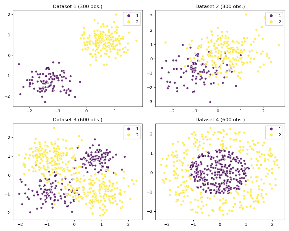
The evaluation is conducted over four distinct, two-dimensional datasets. These datasets were specifically generated to present varying degrees of linear separability and cluster geometries, ensuring the classifiers are tested against a diverse set of decision boundaries.
Models
We selected three distinct classifiers to evaluate varying approaches to the classification problem:
- A K-Nearest Neighbors classifier configured with $k=3$.
- A Support Vector Machine (SVM) utilizing a Radial Basis Function (RBF) kernel ($\gamma=2$, $C=1$).
- A Decision Tree configured with a maximum depth of 5.
Results and Discussion
| RBF SVM | Nearest Neighbors | Decision Tree | |
|---|---|---|---|
| Dataset 1 | 1.000 | 1.000 | 0.995 |
| Dataset 2 | 0.860 | 0.849 | 0.827 |
| Dataset 3 | 0.929 | 0.911 | 0.835 |
| Dataset 4 | 0.976 | 0.970 | 0.959 |
Upon aggregating the cross-validation accuracies and converting them to ranks, the Friedman test yielded a p-value of #strong[0.0224]. Since this value falls below our predefined significance level of $\alpha = 0.05$, we initially reject the null hypothesis, confirming that the performance differences among the classifiers are statistically significant on this specific data split.
However, further analysis revealed that this statistical significance is sensitive to the random_state of the data splitter.
Altering the random seed used to shuffle the datasets (e.g., from 42 to 43) causes the p-value to fluctuate above the threshold to 0.0569.
This indicates that the performance margins between the top classifiers are narrow enough that
the random noise of the train-test allocation heavily influences the final statistical outcome.
This instability is fundamentally caused by the severely limited sample size of $N=4$ datasets,
which lacks the statistical power required for the Friedman test.
To mitigate this variance and obtain a more robust estimate in future evaluations,
it is necessary to evaluate the models over a much larger number of datasets.
Critical Difference Diagram
To intuitively visualize these results, we construct a Critical Difference (CD) diagram. In this diagram, classifiers are positioned on an axis according to their average ranks. Algorithms that do not perform significantly differently from one another are connected by a thick horizontal line representing the CD threshold.
Operating under our primary split to determine exactly where the initial rank differences lie, we applied the Nemenyi post-hoc test, which yielded a Critical Difference threshold of #strong[1.66]. The pairwise comparisons are visualized in .
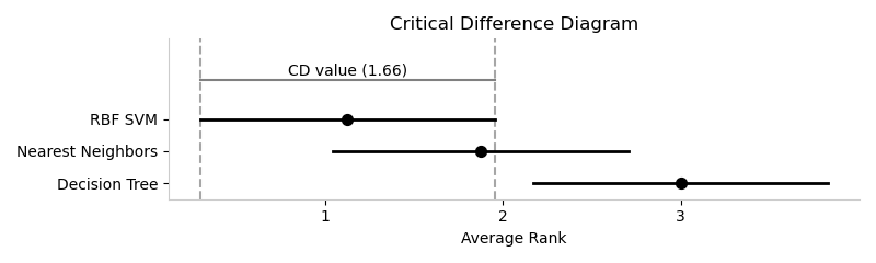
is the Critical Difference diagram
Conclusion
Through the application of a 5-time 2-fold cross-validation and the non-parametric Friedman-Nemenyi pipeline, we conducted a statistically robust comparison of three classifiers. By operating on ranks rather than raw accuracy scores, we successfully mitigated the influence of varying dataset difficulties. The statistical tests, supported by visual evidence from the decision boundaries, conclude that only the RBF SVM significantly outperforms the rigid, axis-aligned approach of the Decision Tree on these specific datasets. The 3 Nearest Neighbors classifier, while visibly competitive, does not exceed the Critical Difference threshold required to claim statistical significance over the Decision Tree.
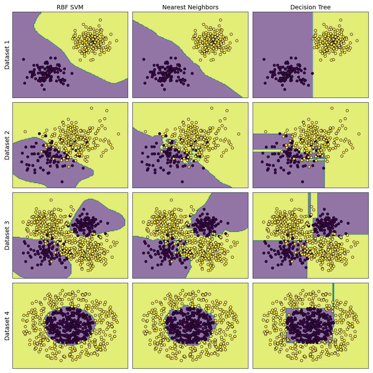
The plotted decision boundaries in provide strong intuition for these statistical rankings. Both the RBF SVM and KNN excel at drawing smooth, continuous, and highly non-linear contours that tightly map the intrinsic distributions of the data. The Decision Tree, however, is constrained by its mechanism of making orthogonal, axis-aligned splits. This limitation forces the tree to approximate smooth curves with rigid, step-like boundaries, ultimately leading to higher misclassification rates and its statistically lower rank in this evaluation.
References
Loading bibliography…